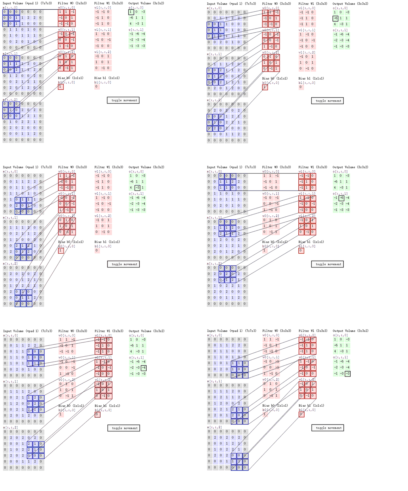
可视化计算网页：https://ezyang.github.io/convolution-visualizer/index.html

1. 一维卷积

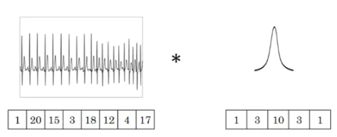
一维卷积主要用于对只有一个维度的时间序列提取特征，比如信号、股价、天气、文本以及自然语言处理领域。

2. Conv Calculation

输入矩阵格式：四个维度，依次为：样本数、图像高度、图像宽度、图像通道数

输出矩阵格式：与输出矩阵的维度顺序和含义相同，但是后三个维度（图像高度、图像宽度、图像通道数）的尺寸发生变化。

权重矩阵（卷积核）格式：同样是四个维度，但维度的含义与上面两者都不同，为：卷积核高度、卷积核宽度、输入通道数、输出通道数（卷积核个数）

adding前面的系数是2，所以在padding时，一般是对称地补，左／右各padding一列 或者 上下各padding一行。stride是2，而括号里算出来的值刚好是奇数怎么办？那就再偷偷摸摸补一列padding或者补一行padding。

• caffe的padding策略是把0补在左上。
• tensorflow的padding策略是把0补在右下。
• padding=1的效果是：原来的输入层基础上，上下左右各补了一行！

输入矩阵、权重矩阵、输出矩阵这三者之间的相互决定关系

$$ H_{out} = \left\lfloor\frac{H_{in} + 2 \times \text{padding}[0] - \text{dilation}[0] \times (\text{kernel_size}[0] - 1) - 1}{\text{stride}[0]} + 1\right\rfloor \ W_{out} = \left\lfloor\frac{W_{in} + 2 \times \text{padding}[1] - \text{dilation}[1] \times (\text{kernel_size}[1] - 1) - 1}{\text{stride}[1]} + 1\right\rfloor $$

• 向下取整 4.9 =4

example one: 标准卷积计算

以 AlexNet 模型的第一个卷积层为例， - 输入图片的尺寸统一为 227 x 227 x 3 （高度 x 宽度 x 颜色通道数）， - 本层一共具有96个卷积核， - 每个卷积核的尺寸都是 11 x 11 x 3。 - 已知 stride = 4， padding = 0， - 假设 batch_size = 256， - 则输出矩阵的高度/宽度为 (227 - 11) / 4 + 1 = 55

tf.keras.layers.Conv2D(
    filters,
    kernel_size,
    strides=(1, 1),
    padding="valid",
    data_format=None,
    dilation_rate=(1, 1),
    groups=1,
    activation=None,
    use_bias=True,
    kernel_initializer="glorot_uniform",
    bias_initializer="zeros",
    kernel_regularizer=None,
    bias_regularizer=None,
    activity_regularizer=None,
    kernel_constraint=None,
    bias_constraint=None,
    **kwargs
)

>>> input_shape = (4, 28, 28, 3)
>>> x = tf.random.normal(input_shape)
>>> y = tf.keras.layers.Conv2D(
... 2, 3, activation='relu', input_shape=input_shape[1:])(x)
>>> print(y.shape)
(4, 26, 26, 2)
################
>>> # With `dilation_rate` as 2.  
>>> input_shape = (4, 28, 28, 3)
>>> x = tf.random.normal(input_shape)
>>> y = tf.keras.layers.Conv2D(
... 2, 3, activation='relu', dilation_rate=2, input_shape=input_shape[1:])(x)
>>> print(y.shape)
(4, 24, 24, 2)
####################
>>> # With `padding` as "same".  
>>> input_shape = (4, 28, 28, 3)
>>> x = tf.random.normal(input_shape)
>>> y = tf.keras.layers.Conv2D(
... 2, 3, activation='relu', padding="same", input_shape=input_shape[1:])(x)
>>> print(y.shape)
(4, 28, 28, 2)
#########
>>> input_shape = (4, 7, 28, 28, 3)
>>> x = tf.random.normal(input_shape)
>>> y = tf.keras.layers.Conv2D(
... 2, 3, activation='relu', input_shape=input_shape[2:])(x)
>>> print(y.shape)
(4, 7, 26, 26, 2)

• padding: one of "valid" or "same" (case-insensitive). "valid" means no padding. "same" results in padding evenly to the left/right or up/down of the input such that output has the same height/width dimension as the input.

• data_format: A string, one of channels_last (default) or channels_first. The ordering of the dimensions in the inputs. channels_last corresponds to inputs with shape (batch_size, height, width, channels) while channels_first corresponds to inputs with shape (batch_size, channels, height, width). It defaults to the image_data_format value found in your Keras config file at ~/.keras/keras.json. If you never set it, then it will be channels_last.

• Input shape

  4+D tensor with shape: batch_shape + (channels, rows, cols) if data_format='channels_first' or 4+D tensor with shape: batch_shape + (rows, cols, channels) if data_format='channels_last'.

• Output shape

  4+D tensor with shape: batch_shape + (filters, new_rows, new_cols) if data_format='channels_first' or 4+D tensor with shape: batch_shape + (new_rows, new_cols, filters) if data_format='channels_last'. rows and cols values might have changed due to padding.

def Generator_model():
    # 下面搭建生成器的架构，首先导入序贯模型
    model = Sequential()
    # 添加一个全连接层，输入为100维向量，输出为1024维
    model.add(Dense(input_dim=100, output_dim=1024))  #100--->1024
    # 添加一个激活函数tanh
    model.add(Activation('tanh'))
    # 添加一个全连接层，输出维128×7×7维度
    model.add(Dense(128*7*7))    #1024-->128*7*7
    # 添加一个批量归一化层，该层在每个batch上将前一层的激活值重新规范化，即使得其输出均值接近于0，标准差接近于1
    model.add(BatchNormalization())
    model.add(Activation('tanh'))
    # Reshape层用来将输入shape转换为特定的shape
    model.add(Reshape((7,7,128),input_shape=(128,7,7)))  #128*7*7-->7*7*128
    # 2维上采样层，即将数据的行和列分别重复2次
    model.add(UpSampling2D(size=(2,2)))                #7*7*128-->14*14*128
    # 添加一个2维卷积层，卷积核大小维5×5，激活函数为tanh，共64个卷积核，并采用padding使图像尺寸保持不变
    model.add(Conv2D(64,(5,5),padding='same'))    #14*14*128-->14*14*128
    model.add(Activation('tanh'))
    model.add(UpSampling2D(size=(2,2)))          #14*14*128-->28*28*124
    # 卷积核设为1即输出图像的维度
    model.add(Conv2D(1,(5,5),padding='same'))    #28*28*124-->28*28*1
    model.add(Activation('tanh'))
    return model

3. 3D 卷积（C3D)

与2D卷积不同之处在于，输入的图像多了一个 depth 维度，即输入为(1, depth, height, width)，卷积核也多了一个k_d维度，因此卷积核在输入3D图像的空间维度（height和width维）和depth维度上均进行滑窗操作，每次滑窗与 (k_d, k_h, k_w) 窗口内的values进行相关操作，得到输出3D图像中的一个value。 针对多通道，输入大小为(3, depth, height, width)，则与2D卷积的操作一样，每次滑窗与3个channels上的 (k_d, k_h, k_w) 窗口内的所有values进行相关操作，得到输出3D图像中的一个value。

4.Paper Reading

level: CVPR CCFA author: Gao Huang ,Cornell University Zhuang Liu Tsinghua date: 2017 keyword:

• CNN

Paper: DenseNet

Summary

1. alleviate the vanishing-gradient problem, strengthen feature propagation , encourage feature reuse and substantially reduce the number of parameters
2. each layer has direct access to the gradients from the loss function and the original input signal,leading to an implicit deep supervision.
3. DensNets require substantially fewer parameters and less computation to achieve state-of-art performance.
4. (CIFAR-10 ,CIFAR-100,SVHN and ImageNet)

• Purpose: to ensure maximum information flow between layers in the network.

Proble Statement

• as information about the input or gradient passes through many layers ,it can vanish and wash out by the time it reaches the end of network . ResNets ,Highway Networks via identity connections; Stochastic depth shortens ResNets by randomly dropping layers; they both create short paths from early layers to later layers

• Traditional feed-forward architectures can be views as algorithm with a state [ResNet] make information preservation explicit through identity tansformations, many layers contribute very little and can in fact be randomly dropped during training.

• Compared to Inception networks,which concatenate features from dfferent laysers, DenseNets

Methods

• system overview:

• Dense connectivit

$$ x_l=H_l([x_0,x_1,x_2,…,x_{l-1}]),x_i\quad refertoI_{layers} \quad output $$

• Composite function:

• Pooling layers: down-sampling layers changing the size of feature maps,refering to layers between blocks as transition layers which do convolution and pooling. the transition layers consist of a batch of normalization layer and 11 convolutional layer followed by a 22 average pooling layer
• Growth Rate: the $l_th$ layers has k0+k*(l-1) input feature-map, k0 is the number of channels in the input layer.
• Bottleneck layers : 11 convolution can be introdeced as bottleneck layer before each 3 × 3 convolution to reduce the number of input feature-maps.
• Compression: reduce the number of feature-maps at transition layers.

Notes 去加强了解

• https://github.com/liuzhuang13/DenseNet
• https://github.com/facebook/fb.resnet.torch
• BN: batch normalization ;ReLU: rectified linear units

level: CVPR author: Kaiming He ,Xiangyu Zhang Microsoft Research date: 2016 keyword:

Paper: ResNet

Summary

Purpose: Deeper neural networks are more difficult to train, a residual learning framework to ease the training of networks

• our extremely deep residual nets are easy to optimize but the counterpart plain nets exhibit higher training error when the depth increases
• easily enjoy accuracy gains from greatly increased depth producing results substantially better than previous networks.

Proble Statement

• Deep networks naturally integrate low/mid/high level features and classifiers in an end-to-end multi-layer fashion,and the level of features can be enriched by the number of stacked layers.

previous work:

• normalized initialization and intermediate normalization layers which enable networks with tens of layers to start converging for stochastic descent with back propagation.with network depth increasing , accuracy gets saturated and thenndegrades rapidly

Methods

• system overview:

Figure 3. Example network architectures for ImageNet. Left: the VGG-19 model [40] (19.6 billion FLOPs) as a reference. Mid- dle: a plain network with 34 parameter layers (3.6 billion FLOPs). Right: a residual network with 34 parameter layers (3.6 billion FLOPs). The dotted shortcuts increase dimensions. Table 1 shows more details and other variants.

Notes 去加强了解

• 去运行一下代码

level: ICCV CCF_A author: Kaiming He ,Georgia Gkioxari Facebook AI Research date: 2017 keyword:

• instance segmentation, bounding-box object detection, person keypoint detection

Paper: Mask R-CNN

Summary

1. efficiently detects objects in an image while simultaneously generating a high-quality segmentation mask for each instance.
2. the method extends Faster R-CNN by adding a branch for predicting an object mask in parallel with existing branch for bounding box recognition.predicting segmentation masks on each Region of Interest(ROI) in parallel with existing branch for classification and bounding box regression.
3. propose ROIAlign that faithfully preserves exact spatial locations

Proble Statement

• R-CNN: Region-based CNN to bounding-box object detection using ROIPool ,Faster-RCNN advanced this stream by learning the attention mechanism with a Region Proposal network . Faster R-CNN consists of two stages. The first stage, called a Region Proposal Network (RPN),proposes candidate object bounding boxes. The second stage, which is in essence Fast R-CNN [9], extracts features using RoIPool from each candidate box and performs classification and bounding-box regression.
• Instance Segmentation bottom-up segments,DeepMask[27] learn to propose segment candidates which are classified by fast R-CNN ; multiple-stage cascade that predicts segment proposals from bounding-box proposals.

Methods

• system overview:

• Mask R-CNN adopts the same two-stage procedure with an identical first stage(RPN),in the second stage .in parrallel to predicting the class and box offset, Mask R-CNN also outputs a binary mask for each RoI.
• Loss Function $L = L cls + L box + L mask$

• we predict m* m mask from each ROI using an FCN[24],allowing each layer in the mask branch to maintain the explicit m*m object spatial layout without collapsing it into a vector representation that lacks dimensions.
• RoIAlign : RoIPool first quantizes a floating-number RoI to the discrete granularity of the feature map, this quantized RoI is then subdivided into spatial bins which are themselves quantized, and finally feature values covered by each bin are aggregated(usually by max pooling) we avoid any quantization of the RoI boundaries or bins (i.e., we use x/16 instead of [x/16]). We use bilinear interpolation [18] to compute the exact values of the input features at four regularly sampled locations in each RoI bin, and aggregate the result (using max or average).

Notes 去加强了解

• Fast/Faster R-CNN[9 29] Fully Convolutional Networ(FCN)
• practice two MaskR-CNN code